
Cloud Observability’s Unified Query Language (UQL) can be used to retrieve and process your metric data. This guide will help you understand how you can use UQL to operate on histogram metrics.
For more details on specific operations, see the UQL Reference. We also have a UQL Cheatsheet to help you build queries.
What is a distribution metric?
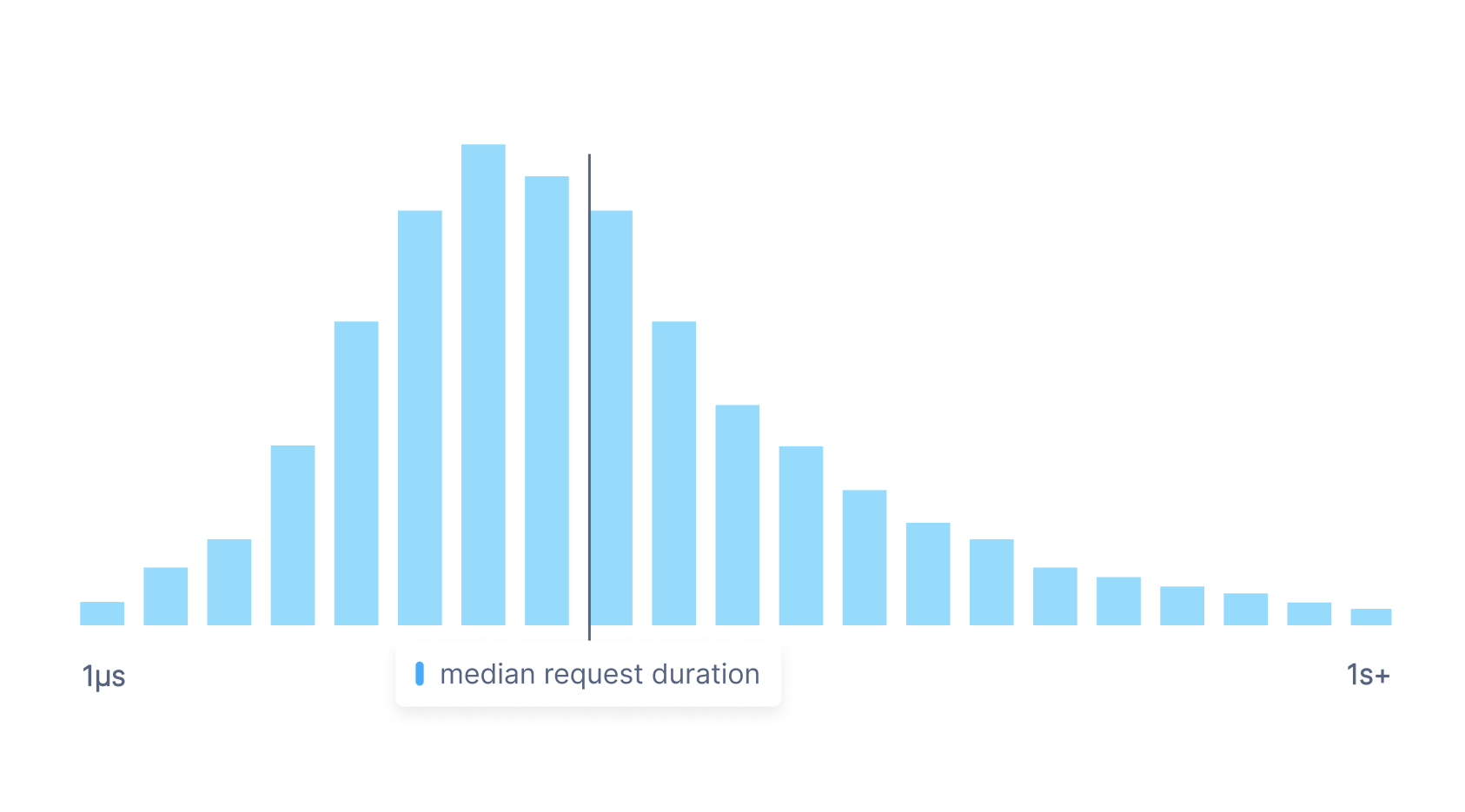
A distribution metric (sometimes also called a histogram) is a metric type that samples value observations, allowing you to approximate individual values for aggregations and calculations in a way that is cheaper than actually storing every individual value. Distribution metrics do this by measuring the frequency of value observations that fall into specific, pre-defined buckets.
For example, if you wish to measure the median latency of requests to a particular service, you can use a distribution metric. Instead of storing all the durations for every single request to the service, you can accurately approximate the true median by storing the frequency of requests that fall into particular duration buckets.
When should you use a distribution metric?
Distribution metrics are useful when you’re not bothered about having the exact values for a time series, but want to be able to perform percentile calculations on a time series without having to capture every value.
Storing distribution metrics is a significantly cheaper and faster way to store and query large quantities of data than storing a scalar metric with a very high number of points.
Querying distribution metrics over a wide time window may take slightly longer than querying scalar metrics over the same time window, because of the size of the distribution metrics.
Using distributions in UQL
Cloud Observability Public APIs currently only support returning scalar time series (made up of int or float values). This means you either must use a percentile, dist_count, or dist_sum point operator or a group_by stage with an appropriate reducer to convert the distribution values into scalar values.
If you are using the Cloud Observability web application with a Heatmap chart type, then you are able to query a distribution metric without transforming the distribution values into scalar values.
Alignment
UQL supports latest aligners for gauge kind distribution metrics and delta aligners for delta kind distribution metrics.
The latest operator will take the latest (or most recent) distribution in the input window.
The delta operator performs a delta alignment across each bucket for each distribution time series in the metric, such that each point in the aligned output distribution metric has a population that does not overlap with other points. Just like with scalar metric time series, you can provide an input window for the delta operator.
Point operators
The percentile point operator operates on the value column of the input time series, calculating the nth percentile for the distribution input, where n is a float value between 0 and 100. You must use the keyword value for the percentile point operator to work on the input distribution metric.
The 90th percentile of response size, summed up by service
1
2
3
4
metric response.size.bytes
| delta
| group_by [service], sum
| point percentile(value, 90)
You can also calculate multiple percentiles from a distribution, producing multiple scalar time series in response.
The 90th percentile, 99th percentile, and 99.9th percentile of response size, summed up by service
1
2
3
4
5
6
metric response.size.bytes
| delta
| group_by [service], sum
| point percentile(value, 90),
  percentile(value, 99),
  percentile(value, 99.9)
Like the percentile point operator, the distribution sum and distribution count point operators operate on the value column of the input time series. The dist_sum point operator calculates the sum of all values within the distribution. The dist_count point operator calculates the total number of values within the population of the distribution.
The average request latency, summed up by service
1
2
3
4
metric request.latency.millis
| delta
| group_by [service], sum
| point dist_sum(value) / dist_count(value)
Aggregation and reducers
There are two reducers to be used with reduce and group_by stages that UQL supports: count and sum.
count returns the count of distribution time series as input (not the total number of values within the population of the distribution)
sum will sum up distribution input time series (not the sum of all values within a distribution). The sum reducer used in a group_by adds together distribution points with the same label value.
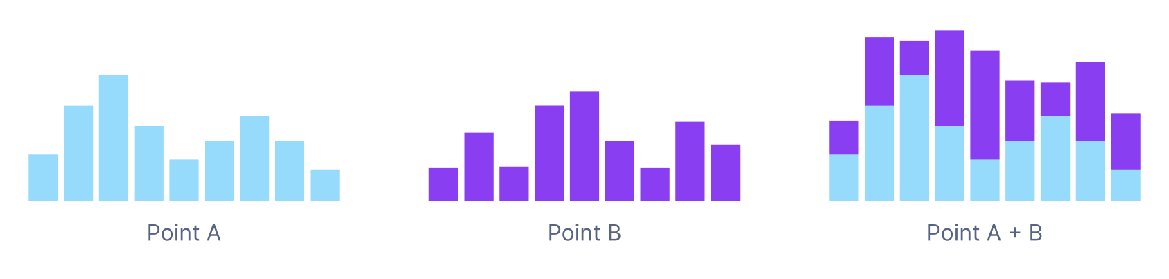
Where one places the group_by statement when querying a distribution is important. The below queries are not equivalent: the first query sums up the distribution points with the same service label, and the second query sums up the 90th percentile of each distribution with the same service label.
1
2
3
4
metric response.size.bytes
| delta
| group_by [service], sum
| point percentile(value, 90)
1
2
3
4
metric response.size.bytes
| delta
| point percentile(value, 90)
| group_by [service], sum
See also
Get started with spans queries in UQL
Updated Oct 4, 2022