
Cloud Observability’s Unified Query Language (UQL) can be used to retrieve and process your metric data. This guide will help you understand how queries are built and illustrate the effects of some common query operations.
For more details on specific operations, see the UQL Reference. We also have a UQL Cheatsheet to help you build queries.
To illustrate the various parts of a UQL query, we’ll walk through two example queries. The final versions of the two UQL queries are:
Request Rate by Service
1
2
3
4
metric requests
| rate 1m
| filter service != "krakend-api-gateway"
| group_by [service], sum
Percentage of total requests by each customer
1
2
3
4
5
(
metric requests | delta 1m | group_by [customer], sum;
metric requests | delta 1m | group_by [], sum
)
| join left / right * 100.0
Query structure
Each UQL query is structured as a pipeline, where each stage of the pipeline happens in-order and runs an operation on the data. In our first example, there are four stages.
1
2
3
4
metric requests
| rate 1m
| filter service != "krakend-api-gateway"
| group_by [service], sum
In our second example, the query starts as two “parallel” pipelines that are merged by the join operation:
1
2
3
4
5
(
metric requests | delta 1m | group_by [customer], sum;
metric requests | delta 1m | group_by [], sum
)
| join left / right * 100.0
Fetch and align metrics
The first stage of any pipeline is retrieving a metric by its name. This can actually be a complete pipeline, but it’s not likely to produce a very useful graph. For example:
All requests without alignment
1
metric requests
This data isn’t sensible without some organization. Metric point writes can come in at any time, and the time interval between points isn’t regular, so it needs to be aligned to an output period. This alignment gives us points at regular intervals, regardless of what the underlying data looks like. It also lets us smooth the data by looking back over a period of time to eliminate noisy variation.
The alignment operators are delta, rate, reduce, and latest. You’ll usually use delta and rate with metrics like a request count, and latest with metrics like “the maximum memory allowed for my program”. See the UQL Reference for detailed information about what situations to use each one in.
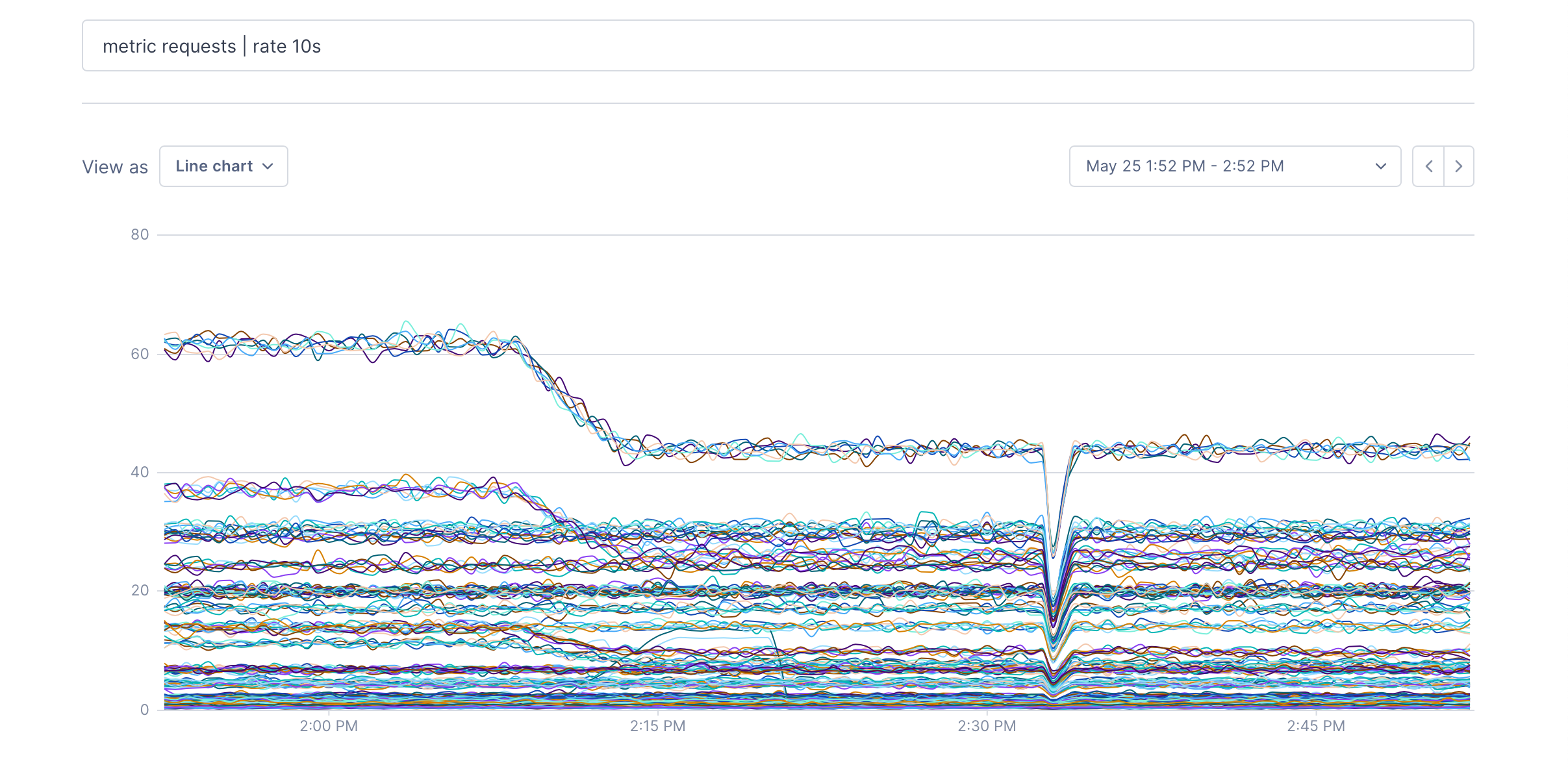
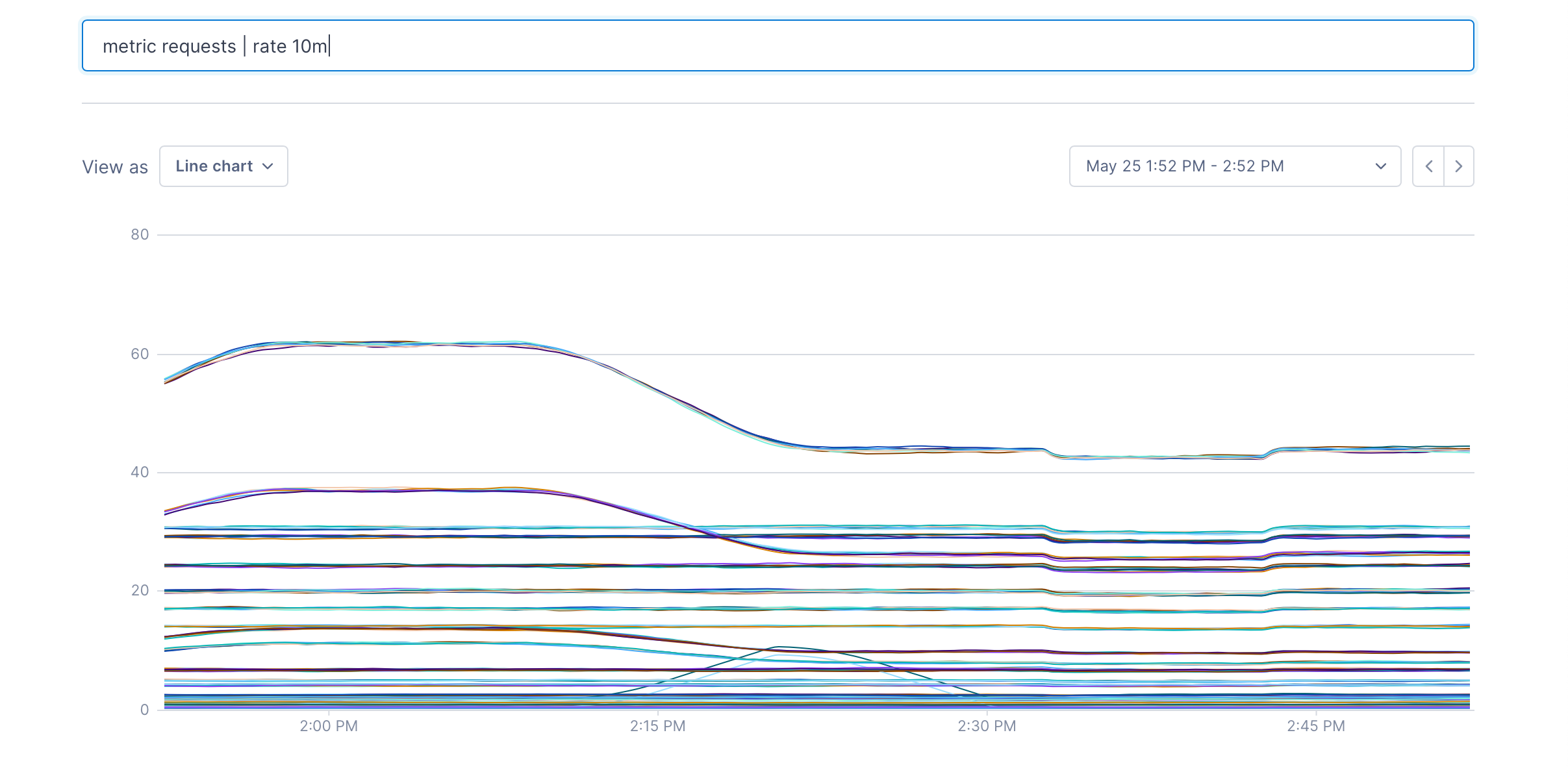
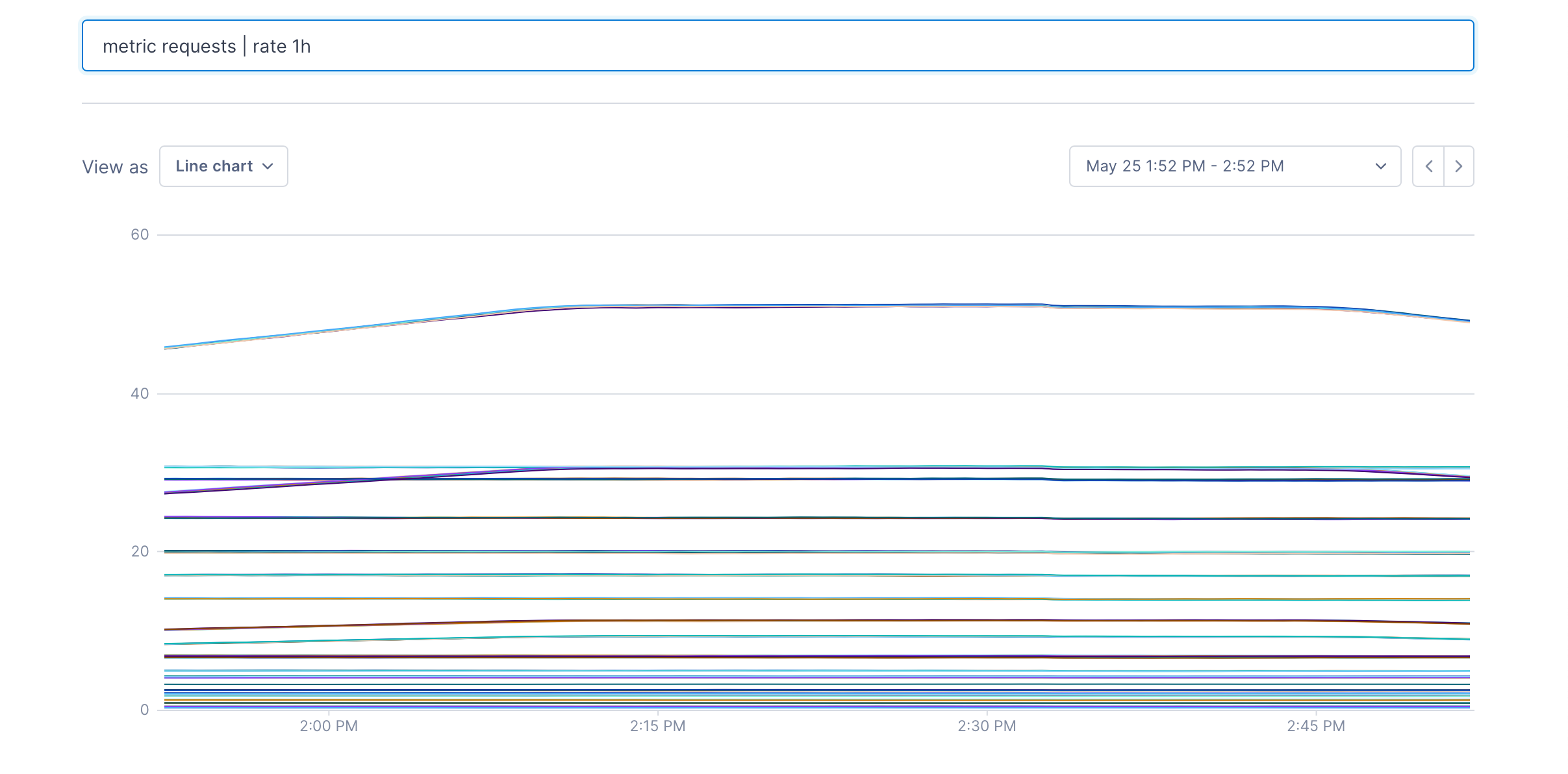
To follow the fetch example, we’ll use rate to add up the requests from each point and produce our output in requests per second.. The argument to rate is the time window; it controls how much data will be incorporated into each point. Longer windows result in smoother output.
metric requests | rate 10s:
metric requests | rate 10m:
metric requests | rate 1h:
Filtering
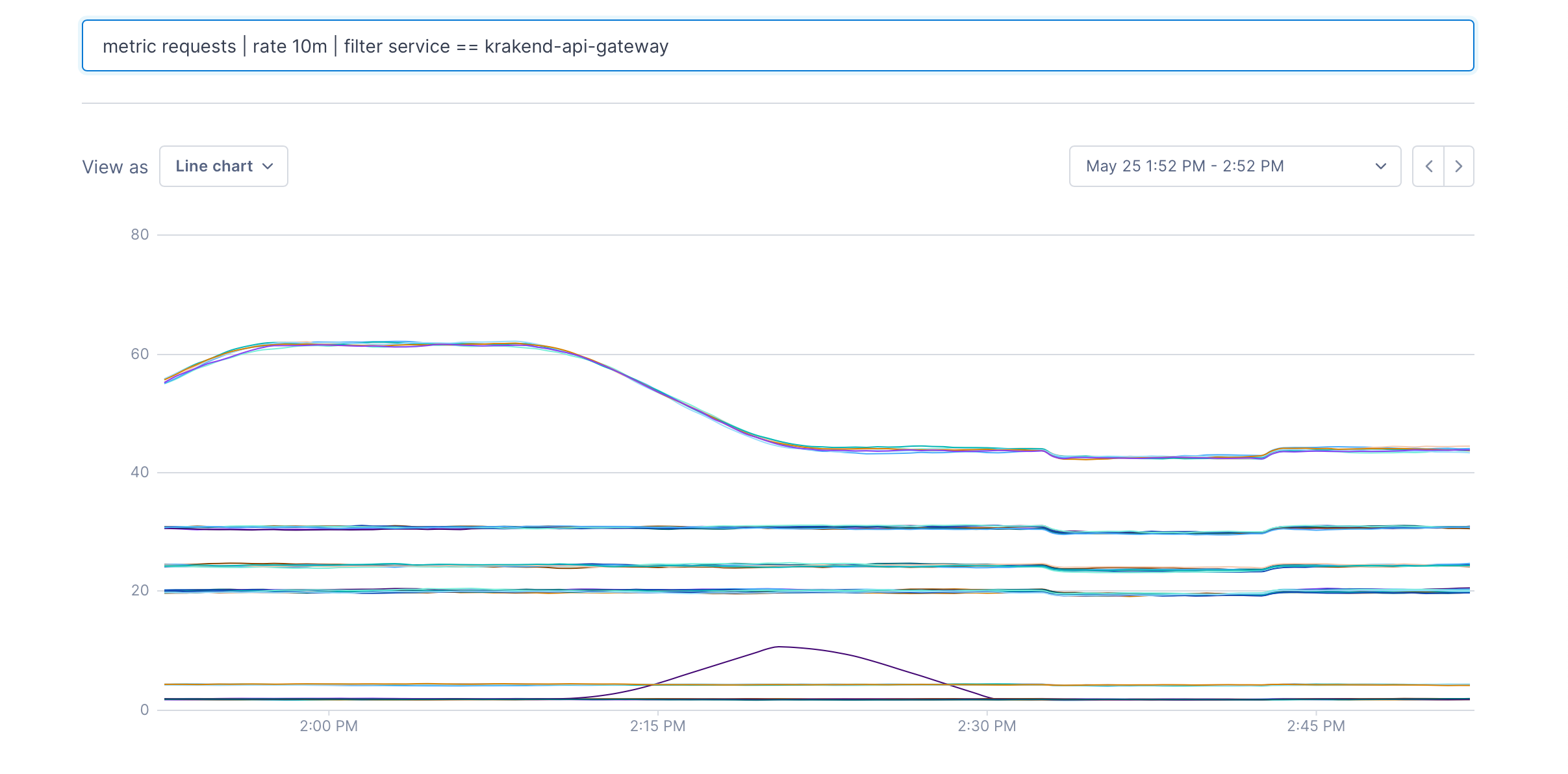
A filter operation can be used to remove metrics from a data set. You write a boolean expression, and any metric that matches the expression will pass through the filter.
After metric requests | rate 10m | filter service == "krakend-api-gateway", only metrics with the label service:krakend-api-gateway will remain:
Grouping
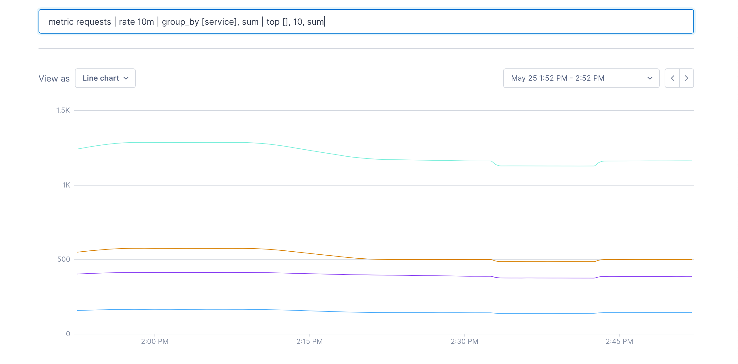
When there are many different metrics in a data set, it’s often useful to reduce the size of the set by grouping them together. We can do this using a group_by operation. Let’s group the result of the query by each service after filtering out the “krakend-api-gateway” service. The [service] argument indicates that each metric with the same value for the service label will be grouped together.
metric requests | rate 10m | filter service != "krakend-api-gateway" | group_by [service], sum
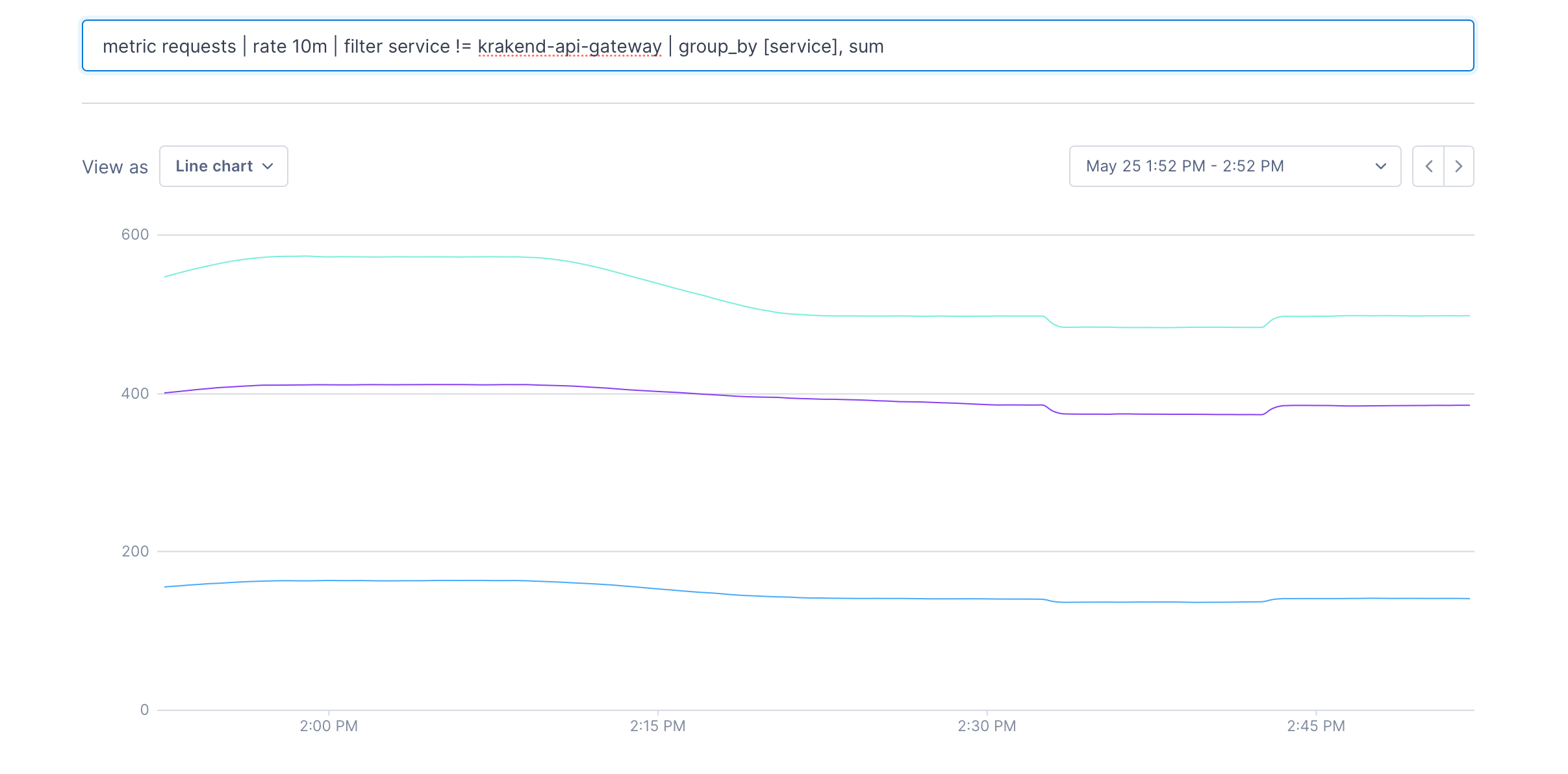
The second argument to a group_by operation is how to group the data in each series as they’re grouped together. The available arguments are listed in the UQL Reference.
Join
Joins are used to combine two separate pipelines according to a formula. They’re very similar to a SQL OUTER JOIN clause. To see how join works, we’ll look at this query:
Percentage of total requests by each customer
1
2
3
4
5
(
metric requests | delta 1m | group_by [customer], sum;
metric requests | delta 1m | group_by [], sum
)
| join left / right * 100.0
and split out the two pipelines inside the ():
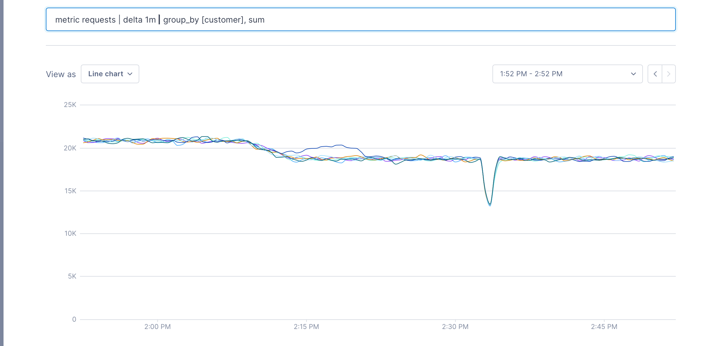
metric requests | delta 1m | group_by [customer], sum
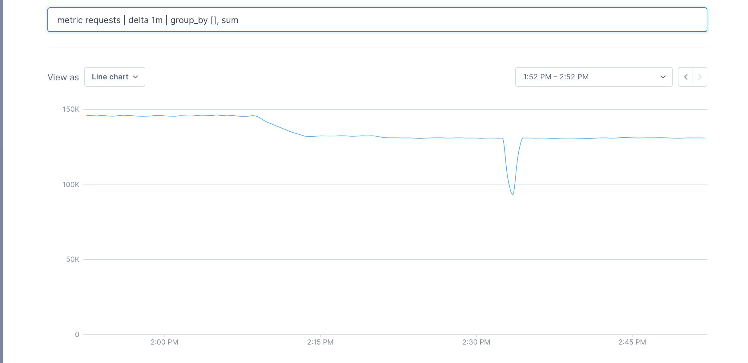
metric requests | delta 1m | group_by [], sum
and the full query:
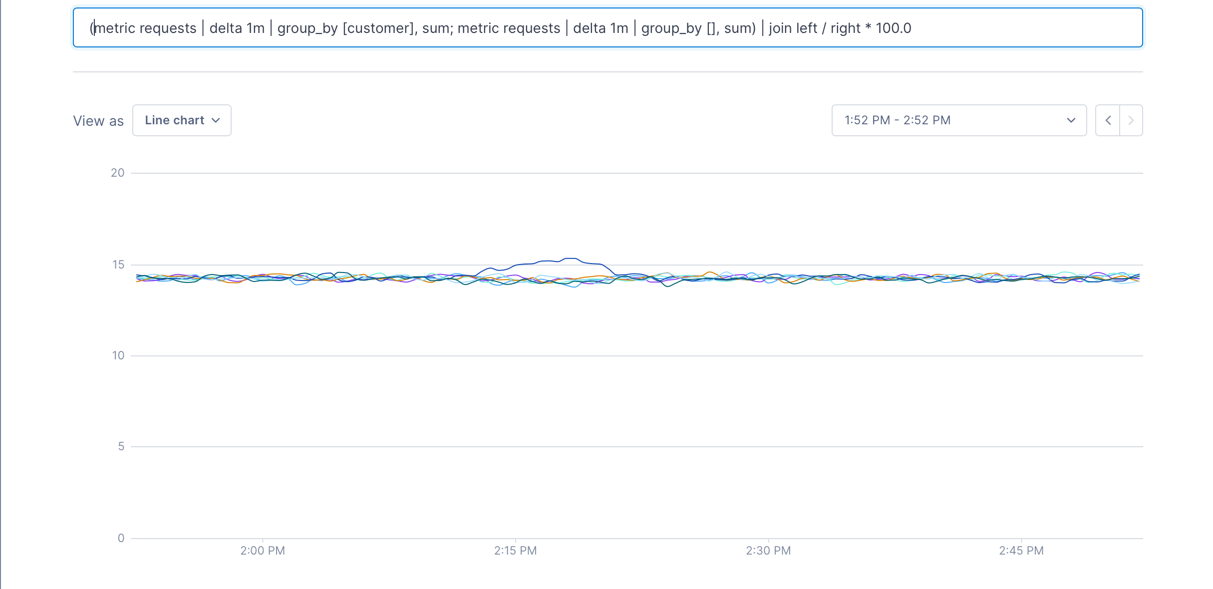
We can see that the first pipeline produces a metric for each customer, and the second one produces a single metric – the total of all requests. When the join is run, we get a metric for each customer that’s the percentage of the total that each customer has issued; in this case, it’s about 14%.
Joins always use the keywords left and right to refer to the two pipelines that they consume. The join’s expression can be any arithmetic that produces a number.
Top and Bottom K
Top and Bottom K operations can be used to reduce the number of metrics in a data set without aggregating them. Let’s say we just wanted the top 10 request metrics, according to the sum of their values.
metric requests | delta 10m | top [], 10, sum
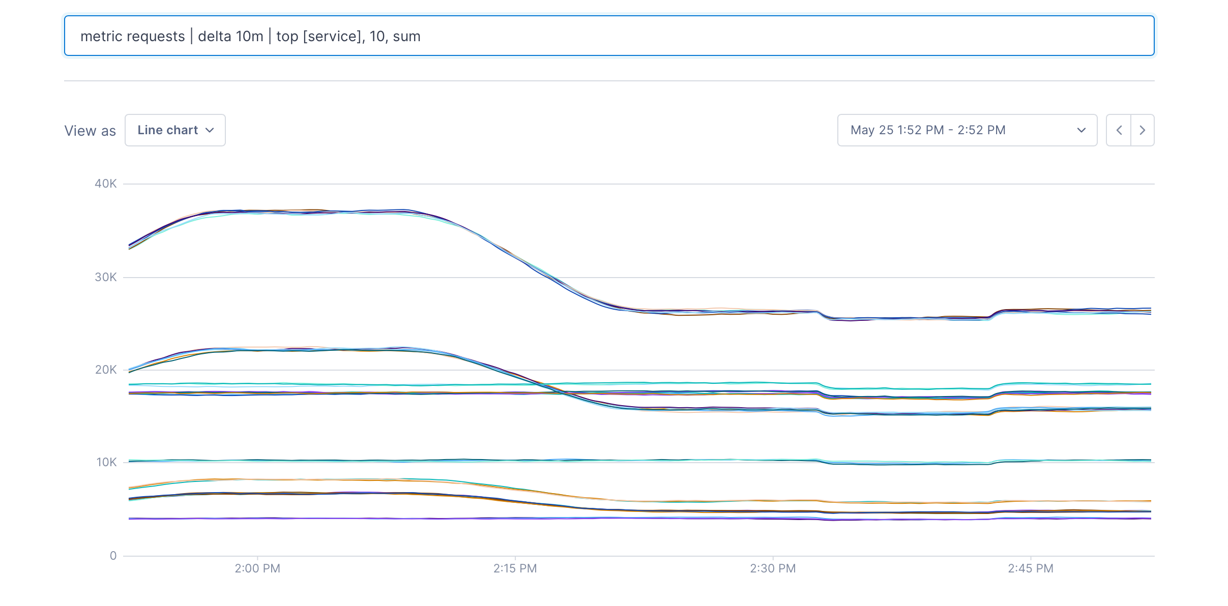
The [] can contain label keys. In this case you get the top 10 metrics for each value of the service label:
metric requests | delta 10m | top [service], 10, sum
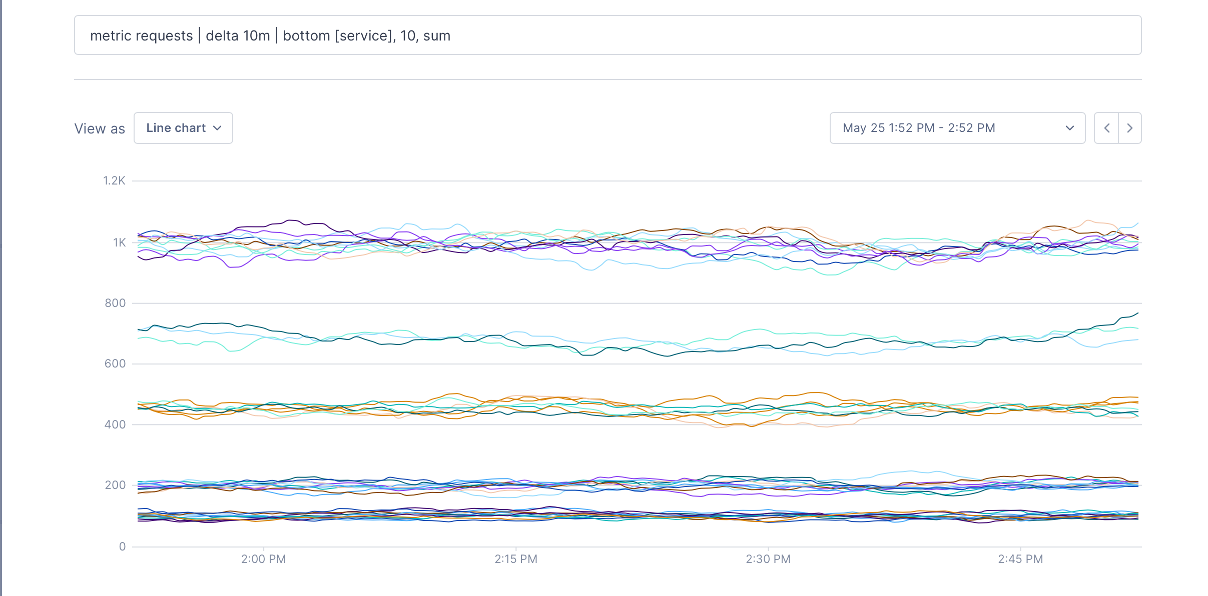
and you can do exactly the same for the bottom 10:
metric requests | delta 10m | bottom [], 10, sum
Point operations
Point operations modify each point in the metric according to a formula. These can be fairly simple operations like value * 2, but they can also be used to transform one type of data into another. We can take a set of integer metrics and turn them into a boolean true/false value:
metric requests | delta 10m | group_by [customer], sum | point value > 1000
This query returns a point with the value true whenever a customers request count is greater than 1000 in the ten minutes before the point.
Time shift operations
Time shift operations allow the points in a time series from a specified period in the past to be shifted forward into the current query evaluation window.
This is useful to easily compare the current values of a time series to values at some time in the past, as it allows time series data from the past to be charted alongside data from the current time window.
For example, to determine if a current load spike is part of a weekly cycle, you can create a chart with a metric and the same metric using a 7d time shift, and visually compare the two lines.
Considerations for alert queries
When creating queries for alerts, keep the following in mind:
- You must set an input window (unless using
latestfor aggregation). - When querying distribution metrics or latency on spans, you can select only one percentage to query on.
- If your query includes multiple sub-queries, you must use a formula to join them and create one output.
- Group-by isn’t supported in alerts.
- To include Regex in metric queries, you must be running this release or later of the Microsatellites.
- Consider adding a final time aggregation to prevent “noisy” alerts.
See also
Updated Oct 4, 2021